5 easy tips to make your excel sheet more organised

Ah Excel, you either hate it or you love it.

However, no matter what side you are on, everyone knows it's a nice software to make overviews in.

If you know how to use it.

And that is a big if. Excel is only as good as the person controlling it.

So I've made a small list of top 5 things for you to make your excel sheet more organised.

In this post I easily explain to you how to make:

1. Drop down menu's

2. If statements

3. Hyperlinks

4. Conditional Formatting

5. Hide sheets and cells

Number 1: Drop down menu's

You may think that this step is already too advanced, but its really easy to make!

This is especially useful if you want to sort your rows under the same category.

Step 1. Make a list of the specifcations in a (seperate) sheet.

Step 2. Go to the cell you want to place your drop down menu in

Step 3. In your nifty search bar at the top, search 'Data Validation'. Usually if you type data you can already find it

Step 4. Well.... click on it.

Step 5. Click under allow 'list'

Step 6. Select your list and press oké

And voilá a beautiful drop down menu. You can use the little box in the bottom right to drag it down and up towards all the cells you want to have this drop down menu in.

Number 2: If statements

If formulas may seem difficult, but they are quite simply in theory. If you wish to analyse something that is a word, simply use "example" and excel will search for the words you need.

An If statement is simple it consists of three parts:

1) what needs to be checked? e.g., is this cell bigger then 10?

2) What happens if it's true?

3) What happens if it's not true?

In that order. See? Easy!

So, for instance, you want to know if a number is higher then 0 because then you want to calculate with it. Then the statement is:

=IF(Cell>0;1;"")

So this says cell F1 needs to be bigger then 0 and then the filled in cell will become 1, the "" means that the cell should be empty.

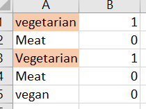
Now, if you want to calculate how many vegetarians there are in your menu or how many tax returns do the same thing, but with the brackets. So:

=IF(Cell = "vegetarian"; 1;0)

It doesn't matter if the cells are written with capitals or not, but they do need to be the same! Good time to try out the drop down menu you now know how to make.

Excel on itself is also very userfriendly with its basic mechanics. If you already type =if then it will show you how to make it:

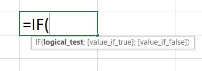
Easy peasy right!

If you want to sum these up, simply use the formula "=SUM() and select the cells you want to sum.

Number 3: Hyperlinks

Hyperlinks can mean between sheets in your own file, other files on your computer or even websites and they are very easy to make!

You can even share a single cell with an e-mailadress. I will leave that for what it is in this post though :p

All of these things start the same:

1) Type what you want in a cell, e.g., overview

2) Right click on the cell

3) Select "link" (Last option)

You will get a page like this, I did remove my file names, I hope you can forgive me:p

On the left you see "link to: Existing file or web page", "Place in this document" and "Create new document".

For the website:

Step 1: Go to the website you want

Step 2: Copy the link

Step 3: Place the link in the Address bar, Make sure that you put www. in front of it, otherwise it won't work.

Step 4: Click ok.

That's it!

For a connection to a seperate folder

Step 1: Know where you saved your file!

You can select in "Look in" in which general folder you put, most likely in documents. If you've just closed it, then click on recent files. You can even select files from e.g., OneDrive, but note that if those files are not on your computer when you don't have WiFi you can also not open them from excel.

Step 2: Select the file

step 3: Click ok

For a link to another cell / sheet

Are you still in the same frame? Good!

Step 1: Click on "Place in this Document"

Step 2: Select the sheet you want to go to, and If needed, specify the ceel in "Type the cell reference"

Step 3: Click ok

And that is three ways to hyperlink to a file, website or seperate sheet!

If you want to make buttons, simply add a shape and follow the same steps.

Number 4: Conditional formatting

Conditional formatting is an easy way to quickly change colours and to see your data.

It's kind of similar to the if-statement.

So I will use the vegetarian/meat example again.

Step 1: Select the cells you want to colour

Step 2: In home click "Conditional Formatting"

Step 3: Select "New rule" at the bottom

You will see this menu:

The one you will use most is the "Format only cells that contain"

So:

Step 5: Select "Format only cells that contain"

From left to right you can select what the program needs to search.

This can be e.g., cell value, Specific texts etc.

The next option is if the value needs to be e.g., equal to, bigger, containing this word etc.

The last option (2 in the example above) are the values. If you click on the button with the arrow, you can select the cell. Otherwise you can type it.

In steps:

step 6: Select which value you want to format

step 7: Select what that value should be

Step 8: Specify the value

Step 9: Press "format..." and select the colour or whatever you want to see if you hit that value. You can specify a lot, so just click around a bit.

Step 10: If you simply want to add a colour, click "fill"

If you want to be extra crazy, you can add a pattern to it via "pattern style".

Example

I want all my vegetarian people to be orange, so I go to my file and select this:

Result?

A perfectly orange selection. If you don't get to see this for all your vegetarian, then your range is probably not set right. Go back to "Conditional Formatting", but this time select "Manage rules", the last option.

Let's continue with the steps shall we:

Step 11: Under "Conditional Formatting" select "Manage rules"

Step 12: Instead of "Current selection" at the top, select "This worksheet".

Step 13: Click on the arrow button under "Applies to" and select the right range.

And there you go! Easy Peasy.

Number 5: Hide sheets

Hiding sheets you don't need or rows can significantly help make your sheet more organized. And it's one of the easiest things to do in excel.

So, e.g., we only want to see how many people in total are vegetarian, but don't really want to see the 1's and 0's.

Step 1: Select the column / row by by clicking on it's name.

Step 2: Right click on it

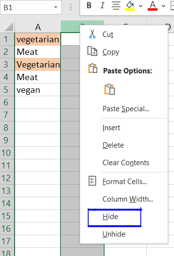
Step 3: Hide

For a sheet it's the same idea. Right click on the name and select hide!

Bonus tip

Suprise! A quick and easy tip, you get for free.

Don't you just hate it when this happens.

There are two easy ways to fix this, well, easily:

On the home page, click "Wrap text"

Or, double click on the rows to make it the exact length of the line.

Sadly, you cannot see my mouse when I take a screenshot, but if you double click on the blue line, shown in the photo below

You will get this:

There we go! 5 easy tips (+1) to make your excel sheets more efficient! If you have any questions or want to read more, please let me know by messaging me.

Thanks for reading and I hope this helps you access your Island life.

---